Dynamic Programming Simplified

What is Dynamic Programming

Dynamic Programming (DP) is a common problem solving technique in computer science. It's dedicated to solve problems having the following properties :

1. Can be broken to smaller pieces called subproblems. Subproblem is as same as the original one, but with "smaller" input, and more importantly, result of the original problem can be constructed from results of subproblems.

2. Those subproblems are overlapping. In other words, there are repeat computations when solving those subproblems. DP can be optimal algorithm in that case, because it can avoid those repeat computations.

Fibonacci number problem

I love simple things. This article is my attempt to simplify DP technique, that why I will choose a very basic problem and solve it with and without DP. And Fibonacci is a perfect candidate for that.

The Fibonacci number is defined by the recurrence relation:

• F(0) = 0
• F(1) = 1
• F(n) = F(n-1) + F(n-2) for n ≥ 2

Problem: given a positive integer n, find F(n)

Let's first solve it without using DP. We can just convert above definition to function with recursive calls. Scala codes :

// file fibonacci.sc
def fib(n: Long): Long =
   if n == 0 then 0
   else if n == 1 then 1
   else fib(n - 1) + fib(n - 2)


println(fib(2)) // output: 1
println(fib(3)) // output: 2
println(fib(5)) // output: 5

Thanks to Scala-cli, we can easily run our codes with the following command :

scala-cli fibonacci.sc

The naive solution works correctly. However, it doesn't scale. With a slightly larger input—say n = 50—running f(50) takes a very long time to complete.

Let’s see if we can solve this using Dynamic Programming (DP).

Step 1: Analyze the Problem

Based on the definition of the Fibonacci sequence:

• F(0) = 0
• F(1) = 1

These are trivial base cases.

Now, let’s look at the general case when n ≥ 2: F(n) = F(n - 1) + F(n - 2)

This clearly shows that we can compute F(n) by breaking it into two smaller subproblems: F(n - 1) and F(n - 2). In other words, we solve the same problem but on "smaller" input.

Also, we can build the final result simply by combining the results of F(n - 1) and F(n - 2).

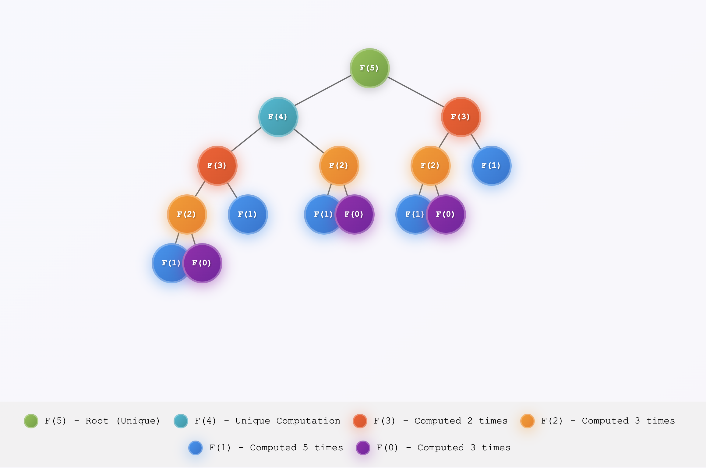
For example, with n = 5, we compute:

• F(4) and F(3)
• Then use them to compute F(5)

However, if you draw the recursive call tree, you’ll notice many duplicate computations. These are shown below as nodes with the same color.

I like to think of it like how all elements in the universe are formed—starting from Hydrogen.

Step 2: Avoid Repeating Work

This observation might seem obvious, but it's crucial for deciding whether a problem can be optimized with DP.

What if we avoid repeated computation by solving F(n - 1) and F(n - 2) first, then using them to build F(n)?

This bottom-up approach is called Dynamic Programming.

To compute F(5):

1. First compute F(2) from F(1) and F(0)
2. Then compute F(3) from F(2) and F(1)
3. Continue this process until we reach F(5)

By doing this, we eliminate redundant computation. The time complexity becomes O(n).

// file: fibonacci-dp.sc
def fib(n: Long): Long =
  def go(i: Int, n1: Long, n2: Long): Long =
    val next = n1 + n2
    if i == n then next
    else go(i+1, n2, next)

  if n == 0 || n == 1 then n
  else go(2, 0, 1)


println(fib(2)) // output: 1
println(fib(3)) // output: 2
println(fib(5)) // output: 5
println(fib(50)) // output: 12586269025

From my experience, I can tell you that most of DP algorithm is just building bottom up like this